Sampling Distributions and the Central Limit Theorem
Section 7.3Today's Plan
See that is a random variable with its own distribution
State the Central Limit Theorem: center, spread, shape
Compute probabilities and percentiles for a sample mean
Sampling Distribution of the Sample Mean
In practice, statistical studies involve drawing a sample and computing numerical summaries, most often the sample mean, .
Different samples from the same population will generally produce different values of . Because varies from sample to sample, it is a random variable with its own probability distribution. This distribution is called the sampling distribution of .
 Interactive
How Good Is Your Memory?
Go to humanbenchmark.com and take the Verbal Memory test.
Words flash on the screen one at a time.
For each word, click "SEEN" if you've seen it before in this session, or "NEW" if it's the first time.
Your score is the number of correct answers before three mistakes.
Nothing to report and nothing to hand in. Just go see what it is.

A Class That Took This Test
36 students. Every dot is one student's score.
 Think about it
Is the Class Average Typical?
That class averaged 40.5. Typical for a class of 36? Or unusually low?
That's a probability question!
We need to know what the distribution of sample means looks like when samples of this size are drawn from the population.
Mean: points
Standard Deviation: points
Skewed right: most scores are modest, a few are huge.
 Discussion
What About the Sampling Distribution of ?
The population mean is points. What do we expect the mean of the sampling distribution to be?
The population standard deviation is points. What about the standard deviation of the sampling distribution? The same? Smaller? Larger?
The population is skewed right. What do we expect the shape of the sampling distribution to be?
Take note of your three answers so you can check them later.
The Central Limit Theorem Machine
Population: the Verbal Memory scores · · · skewed right
Sample size , the size of a class
Draw One Sample
Draw Another. And Another.
Draw 10
Draw 100
Draw 1,000
Draw more samples
Lots of samples of size 36.
Tallest in the middle, falling away evenly on both sides, close to symmetric.
Question 3: The Shape
The sampling distribution of is approximately normal, even though the population is skewed right.
Question 1: The Center
The population mean is 52.
The mean of the sample means lands right next to it. On average, the sample mean equals the population mean: the sampling distribution of is centered on .
Question 2: The Spread
The population standard deviation is 34.6.
The standard deviation of the sample means is far smaller. Averaging 36 scores cancels the highs against the lows, so the sample means are packed in much more tightly than individual scores are.
So What Is the Relationship?
It is not obvious how these two are related.
, Verified
is called the standard error of the mean.
The machine's number is close to 5.77, and it gets closer with more samples.
Three Things We Now Know About
We have the sampling distribution of : every sample of 36 gives a mean, and the means have a distribution of their own.
On average, in the long run:
Smaller: (the standard error)
Normal, even though the population is skewed right
Does the Sample Size Matter?
Same skewed population. Samples of .
Watch the sample means come in.
Not normal. Still skewed right.
Try Samples of 10
Same skewed population. Samples of .
Better. The skew is smaller.
Still not a normal curve.
Samples of 30
Same skewed population. Samples of .
Really beginning to look like a normal curve. The skew is mostly gone.
For most populations met in practice, is enough.
A few extreme ones need more, but 30 is the number we'll go with.
The Central Limit Theorem
Let be the mean of a large simple random sample from a population with mean and standard deviation .
Then is approximately normal, with mean and standard error .
The Central Limit Theorem applies to all populations.
What If the Population Is Symmetric?
A fair die: 1, 2, 3, 4, 5, 6. Every face equally likely. Uniform, and symmetric.
Samples of , the size that failed before.
Already normal.
For symmetric populations, a smaller sample size may suffice.
What If the Population Is Already Normal?
A normal population.
Samples of → normal.
Samples of → still normal.
is just the population itself, and it's normal.
If the population itself is normal, will be normal for any sample size.
When Does the Central Limit Theorem Apply?
EITHER the sample size is greater than 30 …
… OR we have reason to believe the population is normal.
Either one on its own is enough.
If NEITHER holds, we cannot use the Central Limit Theorem to find probabilities.
 Check your understanding
Does the Central Limit Theorem Apply?
Check the two conditions: a large sample, or a normal population.
(a) A simple random sample of size 45 will be drawn from a population with mean and standard deviation .
(a) YES. , so the Central Limit Theorem applies whatever the population's shape.
(b) A simple random sample of size 24 will be drawn from a population with mean and standard deviation .
(b) NO. is not , and we don't know the population is normal.
(c) A simple random sample of size 8 will be drawn from a normal population with mean and standard deviation .
(c) YES. The population itself is normal, so is normal for any sample size.
Computing Probabilities for
Check that (or the population is normal)
Find and the standard error
Same normal curve work as the last section: an area under the curve, or the value that goes with an area
 Example
Example 1: College Student Age
According to U.S. Census data, the mean age of college students is years, with standard deviation years. A simple random sample of 125 students is drawn.
What is the probability that the sample mean age is greater than 26 years?
Does the Central Limit Theorem apply? Then find the mean and standard error of before touching the calculator.
ExampleExample 1: College Student Age
What is the probability that the sample mean age is greater than 26 years?
years
years
Since , we can apply the Central Limit Theorem and use the normal distribution.
Compute and the standard error :
Find the area under the normal curve:


The probability that the sample mean age is greater than 26 years is approximately 0.1197, about a 12% chance.
ExampleExample 2: College Student Age
Same population, same sample: years, years, and a simple random sample of 125 students.
Find the 30th percentile of the sample mean age.
A percentile is a value of , not a probability.
ExampleExample 2: College Student Age
Find the 30th percentile of the sample mean age.
years
years
We know:
The 30th percentile is the value with area 0.30 to its left.
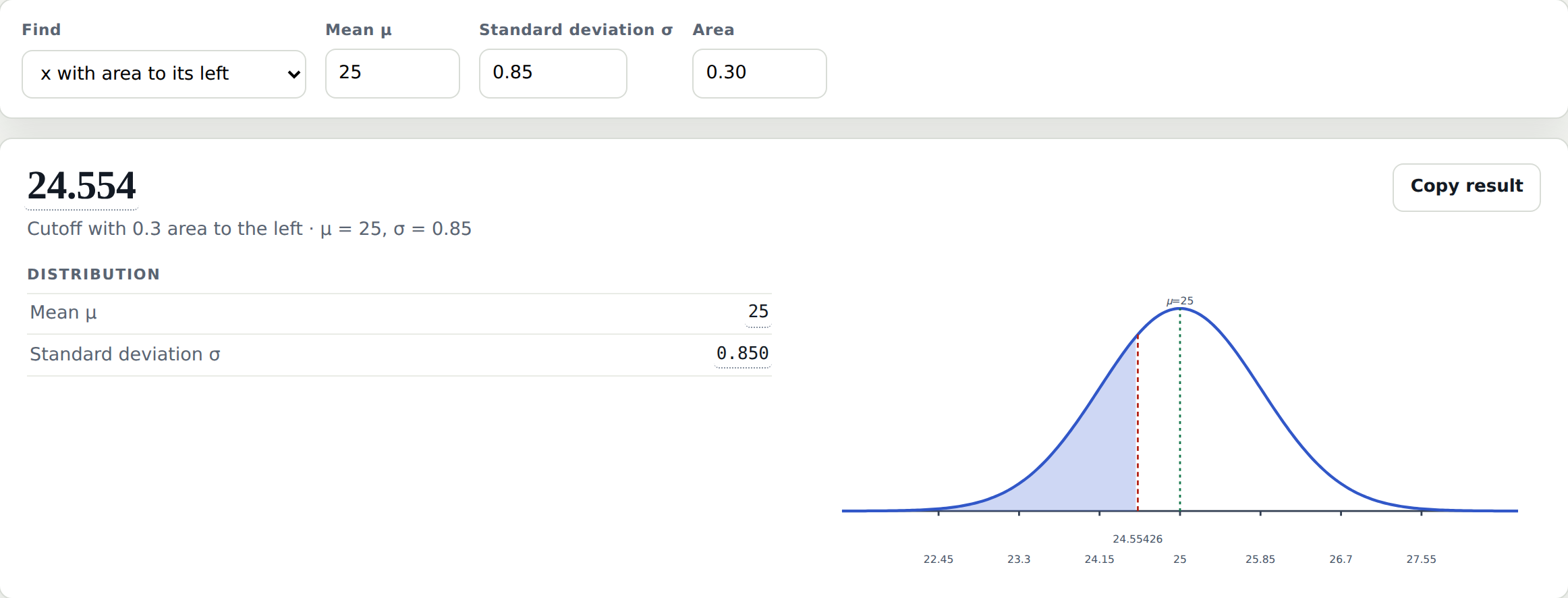
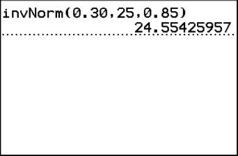
The 30th percentile of the sample mean is approximately 24.55.
ExampleExample 3: Verbal Memory Test
Population Mean: points
Population Standard Deviation: points
The population is skewed right.
Is the sample mean from this class unusual?
Find the probability that a random sample of 36 would have a mean at least as low as 40.5.
If the probability < 0.05 → This class is unusual
If the probability ≥ 0.05 → This class is not unusual
ExampleExample 3: Verbal Memory Test
Is the sample mean from this class unusual?
points
points
Since , we can apply the Central Limit Theorem, even though the population is skewed right.
Compute and the standard error :
Find the area under the normal curve:
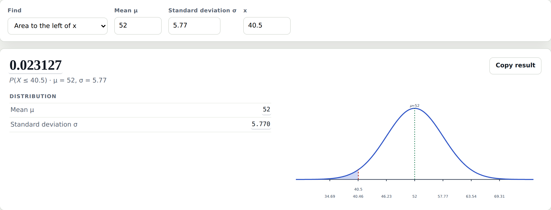
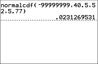
The probability that the sample mean score is less than 40.5 points is approximately 0.0231.
0.0231 is less than 0.05, so this class's average is unusual.
ExampleExample 4: TikTok Usage
Research shows that average daily TikTok usage among teenagers is minutes, with standard deviation minutes. A psychologist samples 50 teenagers.
What is the probability that the sample mean is less than 70 minutes? Would this be unusual?
Two parts: compute the probability, then judge it. “Unusual” means a probability below 0.05.
ExampleExample 4: TikTok Usage
What is the probability that the sample mean is less than 70 minutes? Would this be unusual?
minutes
minutes
Since , we can apply the Central Limit Theorem and use the normal distribution.
Compute and the standard error :
Find the area under the normal curve:


The probability that the sample mean time is less than 70 minutes is approximately 0.0038. It would be unusual.
ExampleExample 5: Food Delivery Times
A food delivery company reports that average delivery time is minutes, with minutes. A consumer group plans to sample 49 deliveries. If the sample mean is unusually high, they will file a complaint.
Above what value would only 5% of sample means fall?
“Only 5% above” means area 0.95 to the left of the cutoff, and the answer is a value of , not a probability.
ExampleExample 5: Food Delivery Times
Above what value would only 5% of sample means fall?
minutes
minutes
We need to find the 95th percentile. Since , we can apply the Central Limit Theorem.
Compute and the standard error :
Only 5% above the cutoff means area 0.95 to its left.
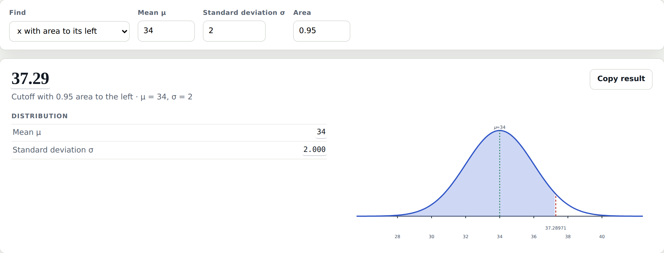
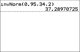
If the sample mean exceeds 37.3 minutes, the consumer group should file a complaint. This would happen only 5% of the time if the company's claim is true.
Case studyThe 18-Minute Claim
Suppose a large airport says the average wait at its main security checkpoint, on weekday mornings from 8:00 to 8:30, is 18 minutes. Waits are skewed right, with standard deviation 12 minutes.
A local newspaper thinks the airport's posted waits run low. Does the evidence show the average is more than 18 minutes?
A reader waited 31 minutes, at 8:15 on a Tuesday.
No. One wait is a single value of .
A reporter times 9 travelers, picked at random in that half hour on different weekday mornings: minutes.
Not enough. Neither condition is met.

A 31-minute wait is not unusual when the standard deviation is 12.
Check the two conditions first.
No,
No, skewed right
Neither condition is met, so the Central Limit Theorem does not apply.
Case studyThe 18-Minute Claim
Does the evidence show the average is more than 18 minutes?
minutes
minutes
The reporter goes back and times 36 travelers the same way: minutes.
, so the Central Limit Theorem applies.
Compute and the standard error :
Find the area under the normal curve:
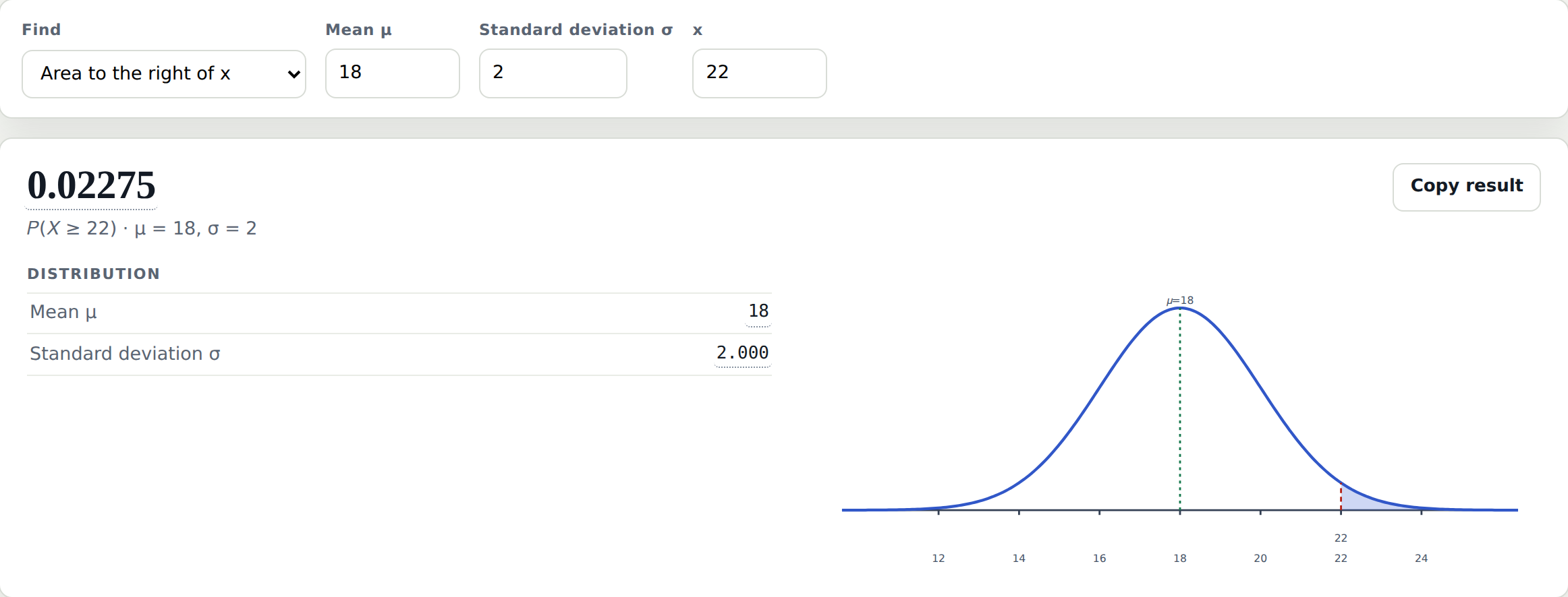
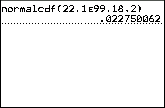
Less than 0.05, so unusual.
Yes. That average would be unusual.
Case studyThe 18-Minute Claim
How high would the average of 36 travelers have to be before we'd call it unusual?
Recall: minutes, minutes, , (the standard error)
Only 5% above the cutoff means area 0.95 to its left.
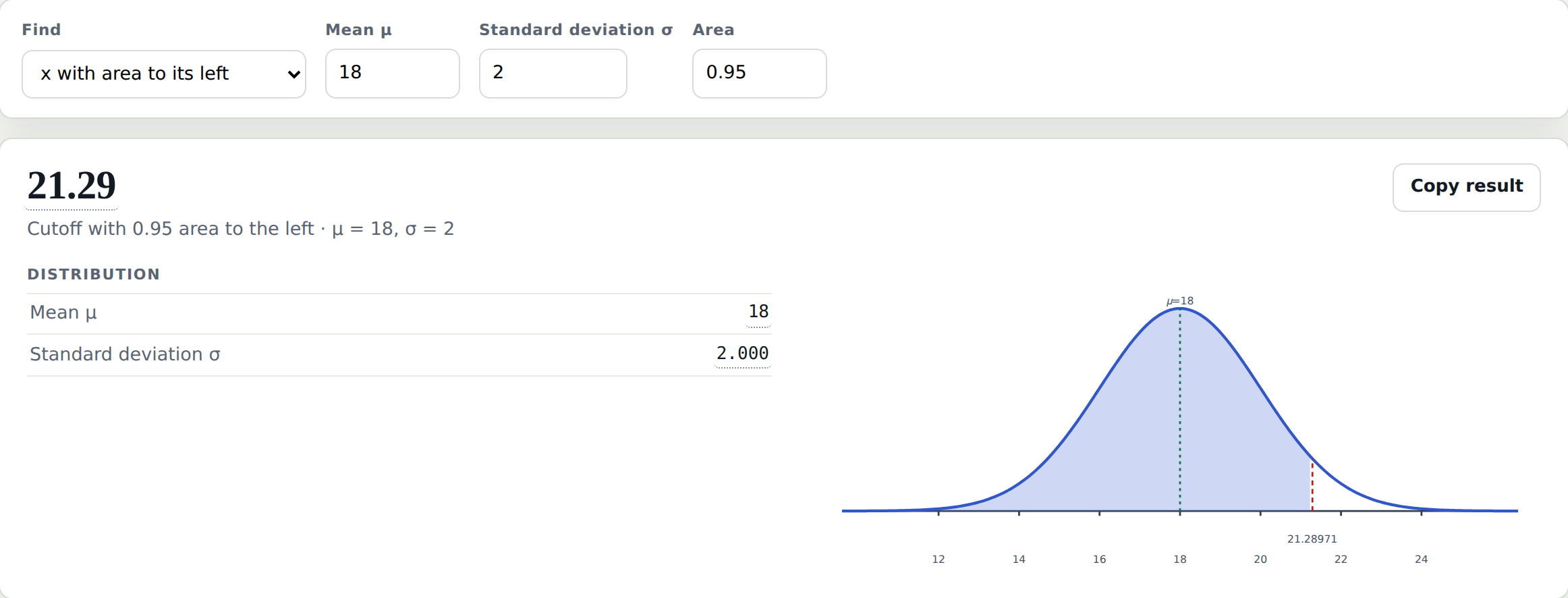

95th percentile of = 21.29 minutes
Any 36-traveler average above 21.29 would be unusual.
Is 21.29 also the 95th percentile of one wait?
No. One wait has standard deviation 12, not 2.
7.3: Sampling Distributions and the Central Limit Theorem
Decide when the Central Limit Theorem applies: , or a normal population
Find the mean of and its standard error: and
Find probabilities and percentiles for a sample mean