The Normal Curve
Section 7.1 & 7.2Use a probability density curve to describe a population
A Curve Built for Mistakes
In the early 1800s, astronomers measuring the same star got different answers every time. Telescopes weren't perfect. The atmosphere interfered.
Carl Friedrich Gauss asked: if every measurement is a little wrong, how do I find the true value?
He developed a curve describing how errors behave. He noted that small errors are common, large errors are rare.

From Stars to Soldiers
Decades later, Adolphe Quetelet applied Gauss's curve to people: heights, weights, chest measurements, waist measurements, blood pressure, reaction times, etc…
Measurement errors can take infinitely many values. That is, they aren’t restricted to a discrete list of numbers.
A probability density curve handles this by assigning probability to intervals rather than individual values.

 Interactive
Continuous Random Variable
Consider a data set consisting of vehicle emissions. We can visualize these data with a relative frequency histogram, with class intervals chosen so each rectangle represents a reasonably large number of vehicles.
Vehicle emissions is a continuous random variable.
Suppose the sample was very large, consisting of millions. Because emissions is continuous, there would be plenty of vehicles for each rectangle even with small class intervals.
 Definition
Probability Density Curve
Such a histogram would look smooth and could be approximated by a curve. The curve used to describe the distribution of this variable is called a probability density curve. The probability density curve tells what proportion of the data falls within a given interval.
Area and Probability Density Curves
The area under a probability density curve between two values and represents the proportion of a population whose values are between and . It can also be interpreted as the probability that a randomly selected value from the population is between and .
Properties of Probability Density Curves
The region above a single point has no width, thus no area. Therefore, if is a continuous random variable, for any number .
This means that for any numbers and .
For any probability density curve, the area under the entire curve is 1, because this area represents the entire population.
The Simplest Case
Before we tackle the normal curve, let's start with the simplest probability density curve: one where every value in an interval is equally likely.
This is called a uniform distribution. The math is just rectangles, which makes it a good place to practice thinking about area as probability.
 Definition
The Uniform Distribution
A uniform distribution is one in which values in any region are equally likely. The probability density curve for a uniform distribution is a horizontal line.
Imagine that when a traffic light turns red, it stays red for 30 seconds before turning green. If you pull up to the light when it is red, the amount of time you will wait before the light turns green is uniformly distributed between 0 and 30 seconds.
 Example
Example: Uniform Distribution
Probabilities for the uniform distribution are straightforward. The probability of an event corresponds to the area of a rectangle.
Find the probability that the waiting time is between 5 and 15 seconds.
The probability that the waiting time is between 5 and 15 seconds is the area of the rectangle with base 15 − 5 = 10 and height , which is .
 Check your understanding
Waiting for the Bus
Buses arrive at a stop every 10 minutes, so the time a rider waits for the next bus is uniformly distributed between 0 and 10 minutes. Find the probability that the wait is
a) less than 3 minutes.
b) greater than 6 minutes.
c) between 3 and 8 minutes.
Use a normal curve to describe a normal population
Normal Curves
Probability density curves come in many varieties, depending on the characteristics of the populations they represent. Many important statistical procedures can be carried out using only one type of probability density curve, called a normal curve.
Normal distributions have one mode and the distributions are symmetric around the mode. Normal curves extend infinitely far both to the right and to the left.
InteractiveProperties of Normal Curves
The mean determines the location of the peak. The standard deviation measures spread. Large values produce a wide, flat curve; small values produce a tall, narrow one.
In a normal distribution, the mean, median, and mode are all equal.
The Empirical Rule
The normal distribution follows the Empirical Rule.
InteractiveAreas Under the Normal Curve
The area under a normal curve represents a proportion of the population or can be interpreted as a probability. It is therefore necessary to find areas under the normal curve other than those specified by the Empirical Rule.
Convert values from a normal distribution to -scores
InteractiveStandardization
The -score of a data value represents the number of standard deviations that data value is above or below the mean.
If is a value from a normal distribution with mean and standard deviation , we can convert to a -score by using a method known as standardization.
The -score of is
Z-scores follow a standard normal distribution, which has mean 0 and standard deviation 1.
Check your understandingConvert to -Scores
The color temperature of LED bulbs from one production line is normally distributed with mean K and standard deviation K. Find the -score of a bulb measured at K.
0.4 standard deviation below the mean.
Find areas under a normal curve
 Calculator
Finding Areas: the Statistics Calculator
On the Statistics Calculator, the Normal tool finds areas under a normal curve. Choose what to find, enter the mean and the standard deviation , and enter the bounds that choice asks for.
https://barrymonk.com/stats-calculator/
 Calculator
Finding Areas: the TI-84 Plus
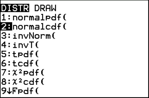
On the TI-84 Plus, the normalcdf command finds areas under a normal curve.
It takes four inputs: lower bound, upper bound, mean, and standard deviation.
Access it by pressing 2nd → VARS.
 Think about it
Example 1: Standard Normal (-scores)
Find the area to the left of .
The value is a -score, so this is the standard normal curve, with mean 0 and standard deviation 1.
1.26 is to the right of the mean, so the area on the left is more than half the curve. Expect an answer above 0.5.
CalculatorExample 1: the Statistics Calculator
Find the area to the left of .
The area we want is on the left, so choose Area to the left of x.
The value is a -score, so the mean is 0 and the standard deviation is 1.
The area to the left of is 0.8962.

 Calculator
Example 1: the TI-84 Plus
Find the area to the left of .
Use normalcdf with −1E99 (or some really small number) as the lower endpoint, 1.26 as the upper endpoint, 0 as the mean, and 1 as the standard deviation.
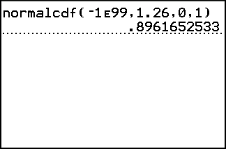
0.8961652533. The area to the left of is 0.8962.
Think about itExample 2: Area Under a Normal Curve
A study reported that the length of pregnancy is approximately normally distributed with mean days and standard deviation days. What proportion of pregnancies last less than 259 days?
The values are in days, not -scores, so the curve is the pregnancy-length distribution itself, with mean 272 and standard deviation 9.
259 days is below the mean, so the area is on the left. It is less than one and a half standard deviations below, so it appears that the area is small, less than 10%.
CalculatorExample 2: the Statistics Calculator
A study reported that the length of pregnancy is approximately normally distributed with mean days and standard deviation days. What proportion of pregnancies last less than 259 days?
The area we want is on the left, so choose Area to the left of x.
We conclude that the proportion of pregnancies that last less than 259 days is 0.0743.

 Calculator
Example 2: the TI-84 Plus
A study reported that the length of pregnancy is approximately normally distributed with mean days and standard deviation days. What proportion of pregnancies last less than 259 days?
We use normalcdf(−1E99,259,272,9).

0.0743070404. We conclude that the proportion of pregnancies that last less than 259 days is 0.0743.
Think about itExample 3: Area Under a Normal Curve
A study reported that the length of pregnancy is approximately normally distributed with mean days and standard deviation days. What proportion of pregnancies last longer than 280 days?
The same pregnancy-length curve as Example 2, but the area we want is now on the right.
280 days is above the mean, so the area is on the right. It is less than a full standard deviation above, so it appears that the area is larger than in Example 2, but still well under a quarter.
CalculatorExample 3: the Statistics Calculator
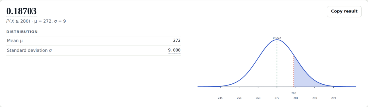
A study reported that the length of pregnancy is approximately normally distributed with mean days and standard deviation days. What proportion of pregnancies last longer than 280 days?
The area we want is on the right, so choose Area to the right of x.
We conclude that the proportion of pregnancies that last longer than 280 days is 0.1870.
 Calculator
Example 3: the TI-84 Plus
A study reported that the length of pregnancy is approximately normally distributed with mean days and standard deviation days. What proportion of pregnancies last longer than 280 days?
We use normalcdf(280,1E99,272,9).

0.1870313608. We conclude that the proportion of pregnancies that last longer than 280 days is 0.1870.
Think about itExample 4: Area Under a Normal Curve
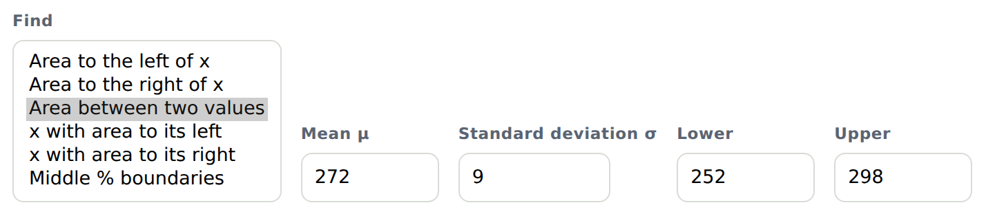
A study reported that the length of pregnancy is approximately normally distributed with mean days and standard deviation days. A pregnancy is considered full-term if it lasts between 252 days and 298 days. What proportion of pregnancies are full-term?
The same curve again, but the area we want now falls between two values rather than in a single tail.
252 days is more than two standard deviations below the mean and 298 days is nearly three above it, so the area between them is almost the whole curve. Expect a proportion very close to 1.
CalculatorExample 4: the Statistics Calculator
A study reported that the length of pregnancy is approximately normally distributed with mean days and standard deviation days. A pregnancy is considered full-term if it lasts between 252 days and 298 days. What proportion of pregnancies are full-term?
The area we want falls between two values, so choose Area between two values.
The proportion of pregnancies that are full-term, between 252 days and 298 days, is 0.9849.

 Calculator
Example 4: the TI-84 Plus
A study reported that the length of pregnancy is approximately normally distributed with mean days and standard deviation days. A pregnancy is considered full-term if it lasts between 252 days and 298 days. What proportion of pregnancies are full-term?
We use normalcdf(252,298,272,9).
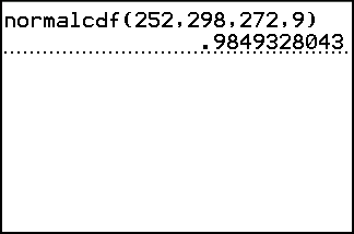
0.9849328043. The proportion of pregnancies that are full-term, between 252 days and 298 days, is 0.9849.
Check your understandingAreas Under a Normal Curve
a) The number of hours a company's employees work remotely each week is normally distributed with mean and standard deviation . Find the probability that an employee works fewer than 12 hours remotely.
b) Waiting times in a clinic are normally distributed with mean minutes and standard deviation minutes. Find the probability that a patient waits more than 53 minutes.
c) Temperature fluctuations in a laboratory are normally distributed with mean degrees and standard deviation degrees. Find the probability that a fluctuation is between and 8 degrees.
Find the value from a normal distribution corresponding to a given proportion
CalculatorNormal Values From Given Areas: the Statistics Calculator
On the Statistics Calculator, the Normal tool returns the value from a normal population with a given area beside it.
Choose which cutoff to find, enter the mean and the standard deviation , and enter the area that choice asks for.

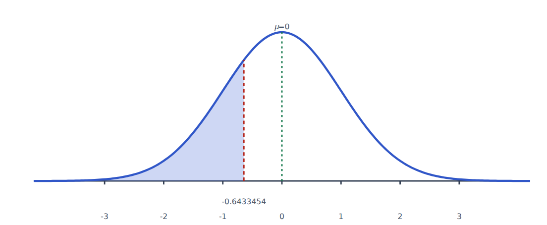
With and , x with area to its left and an area of 0.26 returns the -score with that area to its left.
 Calculator
Normal Values From Given Areas: the TI-84 Plus
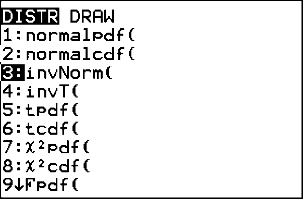
The invNorm command returns the value from a normal population with a given area to its left.
It takes three inputs:
• area to the left
• mean
• standard deviation
Access via 2nd → VARS (DISTR)
 Think about it
Example 5: Finding Normal Values
Scores on an IQ test are normally distributed with mean and standard deviation . What score separates the upper 2% of IQ scores from the lower 98%?
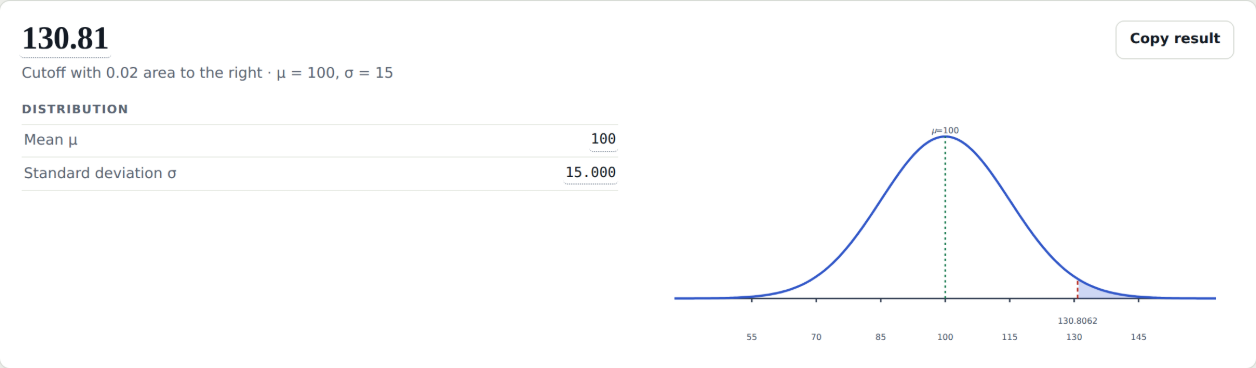
The figure shows the value separating the upper 2% from the lower 98%. Examples 1 through 4 gave a cutoff and asked for an area; this one gives the area and asks for the cutoff.
The area 0.02 is on the right, so the cutoff is well above the mean. Expect a score in the 130s, not one near 100.
CalculatorExample 5: the Statistics Calculator
Scores on an IQ test are normally distributed with mean and standard deviation . What score separates the upper 2% of IQ scores from the lower 98%?
The area 0.02 is on the right, so choose x with area to its right.
We get 130.81. Since IQ scores are generally whole numbers, we round this to .
 Calculator
Example 5: the TI-84 Plus
Scores on an IQ test are normally distributed with mean and standard deviation . What score separates the upper 2% of IQ scores from the lower 98%?
The area 0.02 is on the right, so the area on the left is 0.98.
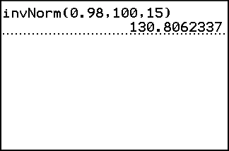
130.8062337. We get 130.81. Since IQ scores are generally whole numbers, we round this to .
Think about itExample 6: Finding Normal Values
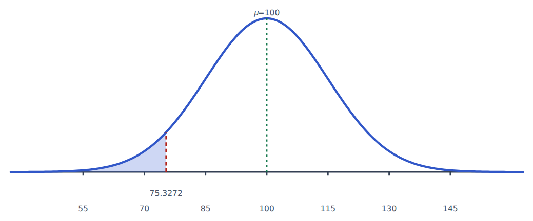
Find the IQ scores that separate the middle 90% of the scores from the top and bottom 5%.
The area is given again, but it is now the middle 90%, so there are two cutoffs to find rather than one.
The middle 90% is centered on the mean, so the two cutoffs fall about the same distance either side of 100, one in the 70s and one in the 120s.
CalculatorExample 6: the Statistics Calculator
Find the IQ scores that separate the middle 90% of the scores from the top and bottom 5%.
The middle 90% falls between two cutoffs, so choose Middle % boundaries.
The middle area is 0.90. That is a proportion, not 90.
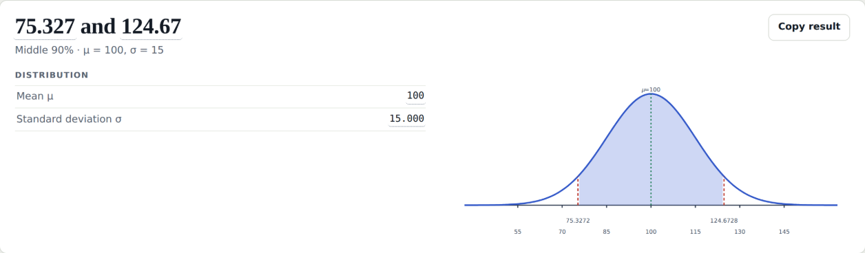
We get 75.33 and 124.67. The middle 90% of IQ scores fall between approximately 75 and 125.
 Calculator
Example 6: the TI-84 Plus
Find the IQ scores that separate the middle 90% of the scores from the top and bottom 5%.
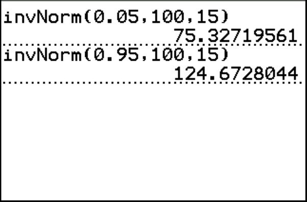
For the lower cutoff, area on left = 0.05. For the upper cutoff, area on left = 0.95.
75.32719561 and 124.6728044. The middle 90% of IQ scores fall between approximately 75 and 125.

 Case study
Will You Make It to Class?
You have two ways to get to campus. Both take 20 minutes on average. Route A is almost always close to it. Route B is all over the place.
We’ll model both as normal: Route A with and minutes, Route B with and .
You leave at 10:35. Class starts at 11:00. Which route gives you the better chance of being on time?
You overslept. It’s 10:45, so you have 15 minutes. Which route now?
Area to the left of 25
On time means the trip takes less than 25 minutes.
Route A · X ~ N(20, 2.5) · P(X ≤ 25) = 0.9772
Route B · X ~ N(20, 5) · P(X ≤ 25) = 0.8413
Same average. The spread decided it. With five minutes of slack, the steady route almost never needs it. The erratic one runs long about one morning in six.
Area to the left of 15
Now on time means the trip takes less than 15 minutes.
Route A · X ~ N(20, 2.5) · P(X ≤ 15) = 0.0228
Route B · X ~ N(20, 5) · P(X ≤ 15) = 0.1587
Neither is good — you’re probably late either way, but Route B gives you the better chance. You need a trip five minutes faster than average, and the steady route essentially never has one.